Statistics and the information they provide are governed by the company they keep. We are conditioned to find them appealing because they seem able to clarify questions through infallible mathematical steps. However, when the wrong question is posed or the wrong group of people studied, no magic wand exists to resolve contaminated data. Although most medical research is done thoughtfully and methodically, it is the practitioner that needs to be able to raise valid objections when warranted, resisting the temptation to apply any given research finding too broadly without analysis.

This article, Part 2 in a new series on interpreting medical research, will teach readers to think critically about the methodology and conclusions of scientific studies. You may wish to refer to Part 1 in the September issue, which lays the groundwork with a series of definitions and concepts that are the stock in trade of medical research. Next month, Part 3 will consider the status and legacy of many landmark studies in eye care. The series will conclude in December with an in-depth look at the output of one prominent research group, the DRCR Retina Network.

The Limits of Evidence

Today, “evidence-based medicine” is the term we use to describe the processes that provide information to doctors indicating that one clinical management choice is better than another not by chance or whim, helping to create what is considered so-called “standards of care.” Studies and reports that make predictive conclusions regarding outcomes of a particular intervention play a major role in determining which procedures, medications and dosages will develop support amongst caregivers and third-party payers. How reliable is this process, and how applicable to everyday practice are the results?

While the discipline of statistics has the potential to provide us with insight and direction on our clinical responsibilities, the calculations and various methods are typically poorly understood, and manipulation can maneuver data toward conclusions that might be ambiguous or distorting to the truth.^1-3 A potential motive might be to bring acclaim to a lab, to justify a research grant (in hopes of securing more) or, for industry-funded studies, to create an advantage in the marketplace. Even well-meaning efforts by honorable people can go awry; bad research need not imply bad intent. Either way, it’s incumbent on us to understand how the data was gathered, sample size determined, who was included and excluded, how the calculations were derived and so on in order to gauge the validity of the conclusions. 

A study’s design and population alone may permit the reader the facility to create inferences about its sensitivity (ability to identify true associations), specificity (ability to rule out spurious associations) or outcomes. A basic understanding of how any study was fashioned, from its premise to its claims, is what permits the reader to determine whether any advice that is offered regarding adjustments in clinical decision making should be followed.^1-3 

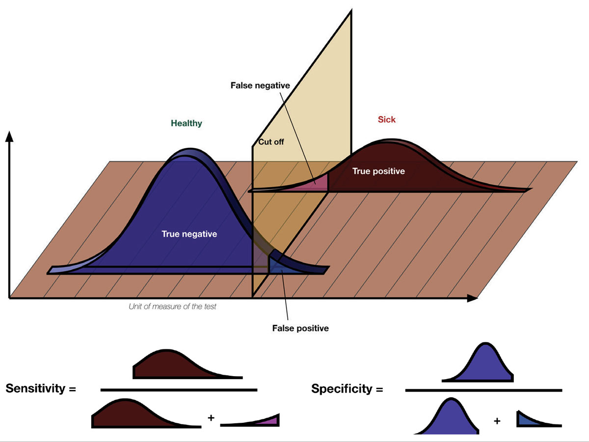
The terms sensitivity and specificity are often used to give credence to research findings. What do they mean? Sensitivity describes the rate of true positives in the data while specificity measures the true negatives. Considering a hypothetical diagnostic test, when there’s a high number of true positives and low number of false negatives, the test has a high sensitivity for the condition in question. A test that reliably excludes individuals who do not have the condition, resulting in a high number of true negatives and low number of false positives, will have a high specificity. Photo: Luigi Albert Maria/Wikimedia Commons.  Click image to enlarge.

We can think of at least five reasons why statistical data may be considered suspect, whether rightly or wrongly: 

1. Different studies can provide different conclusions on the same matter. Rarely is any one study the final word.

2. Interpreter bias creates suspicions of the work. If you dislike the implications of a new finding, you may be more apt to find fault with the study as an avoidance mechanism.

3. The data collection and the sample size were too small, casting doubt on validity.

4. The experimental design was viewed as flawed for the premise of the study.

5. The math was poorly understood by a reader of the study, creating unfounded doubts as to its merit.

In general, associations between variables should be viewed critically; two separate events occurring at the same time do not necessarily imply a cause-and-effect relationship between them. Graphs and charts should be carefully examined. While they are useful tools, scales can be manipulated to make data pictographically more impressive than it is. 

Beware of numbers without context. For example, a news reporter might run with the bulletin: “Blizzard Snarls Traffic—Blamed for 30 Accidents.” However, when all the data are examined, it becomes clear that the average number of accidents on clear days is 50. In this context, the data actually may demonstrate that the storm inhibited accidents by keeping people from driving, actually lowering the number of accidents on that snowy day—completely opposite of what the “alert” implied.

Finally, it is important to realize that small samples are vulnerable to having their results influenced by changes seen in just one or two subjects. While small samples are useful in permitting things to be done quickly and less expensively, bigger sample sizes are more likely to provide analysis that is valid when examining difficult or rare problems.

Types of Studies

Common statistical philosophies in the biomedical literature include descriptive, inferential and Bayesian designs.

Click image to enlarge.

A descriptive study focuses only on the data. It makes no judgements or extrapolations. If we use a coin flip example and the assertion that 50% of outcomes will be heads, a descriptive study would examine the outcome of heads as percentage of the total flips. The descriptive study is a snapshot in time within a set of events. With a sufficient sample size, it might conclude that during this coin-flip session, 50% were indeed heads.

An inferential study attempts to compile information for the purpose of making predictive conclusions extending beyond the collected data. In the coin flip example, after several people carry out the action of flipping the coin, the study might infer that no matter who flips the coin or what type of coin is flipped, 50% of the outcomes will be heads. 

A Bayesian study uses prior information provided from expert observers or previous research and builds upon it. These findings are combined with newly collected data along with other experimental observations to generate new predictions. An example of the Bayesian approach as it relates to the coin flip example might be described as follows: If the coin is placed on the thumb (condition 1) with the head up (condition 2) and flipped using end-over-end technique (condition 3), 50% of outcomes will be heads.

Setting the Scene and Determining the Question

Every experiment or study has an intended purpose: a question that requires an answer. In the field of healthcare, providers generally want to know what causes a condition, its risks and the success rates for various preventions or treatments. To begin any experiment, a question is fashioned; the stated assertion is known as the hypothesis. The rejection of the hypothesis is referred to as the null hypothesis. 

In healthcare, an example question might be, “Does sun exposure increase the risk of skin cancer?” Questions that deal with human physiology are complex because there are many interrelated variables. How do you define sun exposure? Was the individual wearing protective clothing? What were the ethnicities of the study subjects? How were the subjects selected? What were their ages and sexes? Were they wearing sunscreen? What was the sunscreen’s strength?

Even using a coin flip question, which seems much easier, can illuminate the potential for biases: (1) Who is flipping the coin?, (2) Is the coin being flipped always the same coin?, (3) Where is the coin being flipped?, (4) What is the height of the coin flip?, (5) Is the coin always flipped to the same height?, (6) Does the coin’s weight matter?, (7) Are we monitoring the wind during the coin flip? 

The first principle toward understanding how statistical math works is the idea that it is an attempt to prove a counterintuitive. When developing a study, one poses a question (hypothesis) without a preconceived answer and gathers information. The hypothesis is supported only if the subsequent data compel a rejection of the null hypothesis. 

In a different coin flip example, suppose a group convenes to investigate whether the coin that will be used to determine who gets choice of first possession at the Super Bowl is fair. Barring any bias and based upon a lifetime of experience, a reasonable person would expect that 50% of the flips will result in heads and 50% in tails. Posed as a null hypothesis, the question might be written as: “A coin toss sequence with a biased Super Bowl coin will not result in equal outcomes of heads and tails.” In this example, following 1,000 flips, using a flipping machine in a controlled environment, if 500 flips resulted in heads and 500 resulted in tails, the null hypothesis cannot be rejected, leaving by exclusion the conclusion that the coin is fair.

In every study, a researcher hopes to discover new facts. Most experiments are designed to generate data with the assumption that the null hypothesis is true. When the data collected are not consistent with the null hypothesis, the research team is left to conclude the null hypothesis is rejected, making the original hypothesis favored. 

Sometimes, statisticians refer to the hypothesis as the alternate hypothesis. Many experiments fail because the question posed was faulty or ill-defined. Some fail because the data collected answered a question that was not proposed as part of either the null hypothesis or alternate hypothesis. Some fail because the method of answering the question was faulty. Good experiments possess clear, definitive questions and use standard methods of data gathering.

Fig. 2. Examples of corneal surface and tear film effects of neurodegenerative diseases: (A) corneal epithelial erosions, which stain positive with fluorescein, (B) inspissated meibomian glands, which can undergo in-office expression, (C) atrophy and dropout of meibomian glands. Click image to enlarge.

Risky Business

When formulating questions pertaining to living things, it is important to know how common an ailment is among certain populations and the likelihood that it will occur. Risk (denoted in statistics by the letter “p”) compares the number of subjects in a group who experience a new event in proportion to the total number of subjects in the group, determined as follows:

P = n_event /n_total

Risk represents the probability that the new event will occur to a member of that group. When risk is calculated over a given time frame, it is termed the incidence (new cases/time). Incidence is a measure of the rate at which the event occurs. There are various factors that enhance the chances of an outcome (e.g., getting a disease). These factors increase the risk. For example, smoking and heredity are known to increase the likelihood of acquiring age-related macular degeneration (AMD). When an individual has risk factors, they are said to have exposure. The term relative risk (RR) predicts the chances of disease in an exposed group vs. to a non-exposed group. An eyecare example might be, what is the relative risk of acquiring AMD by the “exposure” obesity? Expressed as follows:

RR = P_exposed /P_{not exposed}

Prevalence defines the number of individuals found to have the condition being studied as a proportion of the total population at any given time, whereas incidence is linked to a fixed time period, usually one year. It is a study of penetration. Prevalence is a proportion, not a rate.

Measures of Central Tendency and Variability

We’re all familiar with the terms mean (average value), median (middle value), and mode (most frequent value) as mathematical measures of data sets. For an equally distributed data set, the mean is an accurate measure of the center. However, it is subject to extreme values. In skewed distributions (those with outliers), the mean may not accurately describe the middle. If so, the median may be more appropriate. The mode can be used descriptively but not in calculations. 

The mean by itself is helpful; however, it can be more descriptive when coupled with a measure of variability, or spread of the data. The two most common are the standard deviation (SD) and the confidence interval (CI).

In an eyecare example, given a set of intraocular pressure (IOP) measurements taken on one eye of a subject, suppose the values (in mm Hg) over a 24-hour period were 13, 12, 15, 16, 20, 19, 20, 17, 16 and 15. The standard deviation is the average variance from the mean, both higher and lower. The mathematical representation is somewhat complicated (symbolically and functionally). It can be calculated easily by entering the data into an SD calculator. 

Here, the mean IOP is calculated to be 16.3mm Hg and the standard deviation equals ±2.75mm Hg. Now, as we examine the data, two-thirds of all the measurements are within one standard deviation (2.75mm Hg) from the mean (16.3mm Hg) and 95% of the measurements are within two standard deviations (±5.50mm Hg) of the mean. We can conclude that this patient has an IOP between 13mm Hg and 19mm Hg two-thirds of the time.

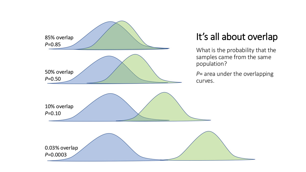
The confidence interval is expressed as a decimal that lies between 0 and 1. It represents the percentage of time the value generated by the experiment satisfies the null hypothesis. There are several ways researchers report this. They may state p<0.05 or p=0.05. These mathematical statements mean that when the data is analyzed, less than 95% of the time does the outcome satisfy the null hypothesis—or 95% of the time, the hypothesis is true. Though it is left to the investigation team, the probability range for the confidence interval is traditionally 0.95 or p<0.05. 

Why 95? As the story goes, Ronald Fisher, one of the founders of statistical mathematics, debated with himself the margin of error he could accept regarding crop fertilizer comparison studies. A 10% margin of error seemed too expensive—losing one out of every 10 crops because the fertilizer he used was worse than the year before—and a 1% margin was too constricting (losing one out of every 100 crops at the expense of trying new fertilizer that might help his business). After some experimentation with the math, he recognized that a 5% loss matched two standard deviations away from the mean (losing one crop out of every in 20) and he reasoned this was an acceptable risk against the possibility of returns with better yields when the new fertilizer was better. Thus, the 5% value, p<0.05, was adopted as the convenient cut-off for a significant deviation from the expected result. 

The scientific community adopted this cut-off with the same logic for non–life-threatening issues. However, different choices are common in other contexts. Many vaccines have rare but serious adverse effects, including meningitis and death. Public health officials do not consider 5% risk of death acceptable. Field trials for vaccines require safety profiles with less than one serious outcome per million (p<0.000001).

Since the confidence level is selected by the experimenters, a given study must be carefully evaluated. A wide confidence interval, such as p<0.05, says the null hypothesis is satisfied less than 5% of the time. This permits researchers to reject it. A wide confidence interval helps to lend great credibility to the hypothesis. This is why it is important at the start of any study to understand the question of the study and to ensure the study is designed to resolve the question at hand.

Answering questions with regard to people is much more difficult than with crops. Trying to determine if a particular visual field or OCT result is normal or pathologic is not only complicated because there are so many variables, but the implications on an individual’s management and functioning may hang in the balance.

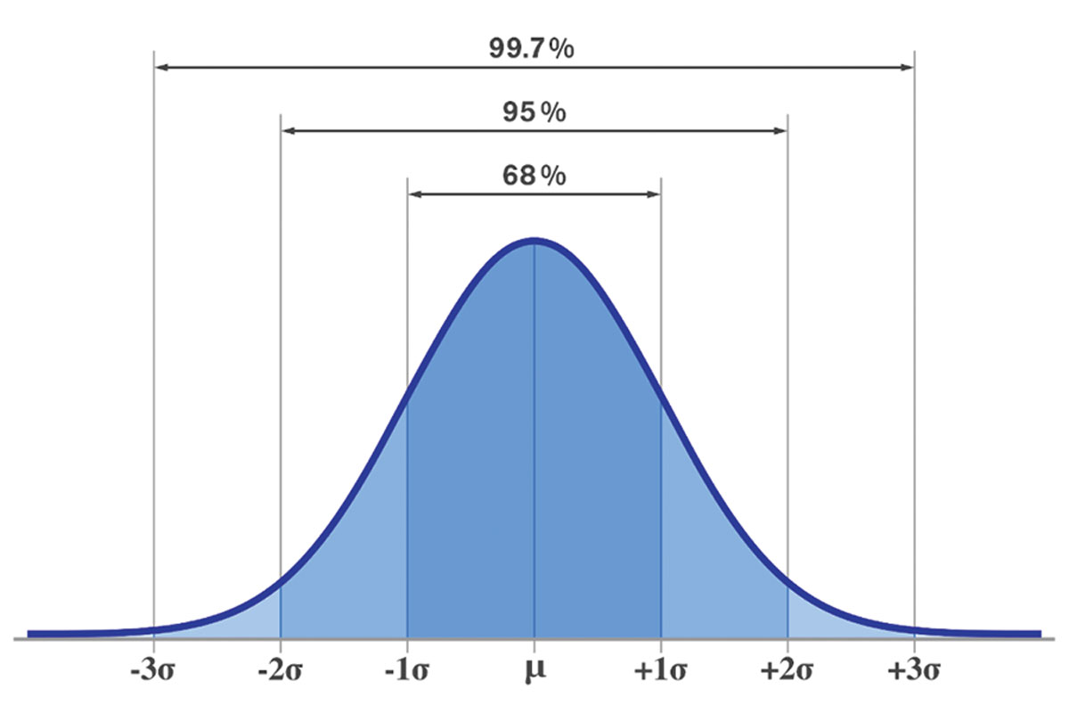Standard deviations are fixed intervals from the mean in a data set that describe results that fall within 68% (SD1), 95% (SD2) and 99.7% (SD3). A higher SD value means there is more spread of the data—and thus less reliability in the relationship they describe—while a low one means more values fall closer to the mean. Click image to enlarge.

Impact of Sample Characteristics

Experimental design fosters fairness. This means the study should include the appropriate subjects or what is often referred to as a representative sample from the group or population of interest. The sample space is the location from which the sample of the population will be taken. Are these appropriate conditions for gathering clinically relevant data?

To eliminate selection bias, the sampling method must pick participants from a target population randomly—we are not necessarily interested in how a glaucoma medication works in everyone, just in people with glaucoma. After the initial selection, inclusion and exclusion criteria specific to the experiment can be used to regulate who is permitted to participate. As an example, for a study examining the conversion rate to glaucoma, subjects already diagnosed with the disease should be excluded. 

When a group is convened to participate in an experiment, it becomes a cohort. The cohort shares the experience of the experiment together.  

A common skepticism in medical research occurs when a representative sampling is acquired internally from a specialty clinic. A practice specializing in glaucoma therapy will likely have glaucoma suspects and patients with particularly high risk. Critics might argue that these patients do not represent “average” glaucoma suspects across typical eyecare clinic populations and certainly do not represent a non-clinical population. Here, an inappropriate sample space might cause skewed results and raise questions about the validity of the study due to flawed experimental design. 

The term that relates to the number of subjects in an experiment is known as the sample size (n). Demographics are important whenever an experiment is completed with living things: the age, sex, race and ethnicity of the subjects, their relative state of illness or wellness, their insurance status and other factors affecting access to care are among the most common factors to contemplate when evaluating a study’s sample. The larger the sample size, the more its variability will be reduced.

We see such effects come into play not only in clinical studies but sometimes in the tools used in the studies themselves. For instance, the phenomena of “red disease” (false positives) and “green disease” (false negatives) in OCT testing have brought greater scrutiny to these devices (where some clinicians read the “color interpretation” of the data without analyzing the actual numbers). Manufacturers scan a variety of individuals across the variables of age, race and sex to arrive at a database that can be used for comparison to your specific patient in the clinic or a subject in a study. Are these truly representative of the global population? These used to be called normative databases, but the terminology has lately moved to the more neutral reference databases to remove the implicit validity in the word normative. 

Hypothesis Testing

Valid conclusions based on statistical calculations depend on properly formed questions to be tested, identifying a study population, gathering an adequate and appropriate sample from that population (by selecting study participants that apply to the hypothesis) and making the selection from an appropriate sample space. 

Time and cost are significant limiting factors in every experiment. The larger the sample size and the longer the experiment is conducted, the more expensive it will be. Unfortunately, sampling large populations is preferred because they estimate or approximate how the entire population would behave. 

When sample sizes are small (n<30), the t-distribution is used. A z-distribution is used when sample sizes are large and when the variance and standard deviation are known. When sample sizes approach 100 (n=100), the two distributions become mathematically indistinguishable. When these distributions are graphed, they define what is referred to as the bell-shaped curve. The confidence interval selects the upper and lower boundaries underneath the curve. Any data that does not fall within the confidence interval is said to fall under a tail (low values to the left, high ones to the right). 

What is not obvious is that large sample sizes are a double-edged sword. For example, a new drug for reducing intraocular pressure is compared to a standard drug in a clinical trial. In a smaller sample study (n=97), the mean reduction in IOP for drug A was 5.2mm Hg and for drug B was 4.8mm Hg, resulting in a p-value of 0.35 (the drug fails to provide a difference in IOP-lowering effects 35% of the time). In a larger study (n=2,500) the mean IOP reduction was 5.0mm Hg for drug A and 4.7mm Hg for drug B, leading to a p-value of 0.05. With this data, the manufacturer can then advertise that drug A is statistically better at reducing IOP than drug B by a wide margin (the drug only fails to provide IOP lowering 5% of the time)—a rather convincing claim. 

However, by examining the data, the astute clinician can ask the question, “By how much is the IOP lower 95% of the time?” What if the data demonstrate the difference is 0.3mm Hg, as in the example above? Is that so earthshakingly good that it is worth switching to the new drug? What if drug A costs twice as much as drug B? What if drug A is not covered by the patient’s insurance plan?

Finally, all studies must have a definitive length. This must be delineated at the outset with any change parameters defined. 

Conclusions and Questions

Evidence-based conclusions help to create standards of care; we are better off with these guidelines than without them. The evidence-based model provides us with insights that are not always possible through our own anecdotal experiences from practice and it aides in drug and device approvals used to treat our patients. The creation of the Food and Drug Administration in 1906 did away with the infamous snake-oil salesmen, who plied their wares with trickery and persuasion rather than facts. We can now rely on objective data, described (ideally) in a transparent way for others to criticize and build upon. But this shift does not absolve us of responsibility to think for ourselves. 

Keep the above questions and caveats in mind to guard against misinterpretations and biases whenever medical research is offered as a way to help you become a better clinician.

Dr. Gurwood is a professor of clinical sciences at The Eye Institute of the Pennsylvania College of Optometry/Salus at Drexel University. He is a co-chief of Primary Care Suite 3. He is attending medical staff in the department of ophthalmology at Albert Einstein Medical Center, Philadelphia. He has no financial interests to disclose.

Dr. Hatch is chief of the Pediatrics and Binocular Vision Service at The Eye Institute of Pennsylvania College of Optometry/Salus at Drexel University. He has no financial interests to disclose.