 |
In July, Review of Optometry celebrated its 125th anniversary. Upon the occasion, I took a look back at decades of published articles on glaucoma and evaluated their clinical relevance today. Now, I’m taking some time to reflect upon the 30 years that I personally have spent in practice. In that era, we’ve witnessed tremendous changes in glaucoma care—and it’s not over yet.
Here, I discuss how glaucoma care has changed in 30 years and what developments currently in the pipeline will become the norm in monitoring these patients in the future.
The Way We Were
When I began practice in 1985, the diagnosis and management of glaucoma was simple. In hindsight, this was probably due to lack of knowledge about the disease’s nuances and risk factors complicating matters. Back then, we initiated treatment on patients who had elevated IOPs, suspicious disc findings and visual field defects. In cases where field defects were not detected, we often deferred treatment until an IOP threshold—usually 30mm Hg—was reached. Research already showed black patients generally had larger optic nerves and, therefore, larger optic cups. We also thought that normal tension glaucoma was relatively rare. We didn’t yet know the role that corneal thickness played, especially in black patients, nor were we fully on board with the concept of preperimetric glaucoma (glaucomatous damage that was present before visual field aberrations). In fact, the earlier definition of glaucoma as proffered by the American Academy of Ophthalmology included references to elevated IOP, optic nerve damage and visual field defects.1
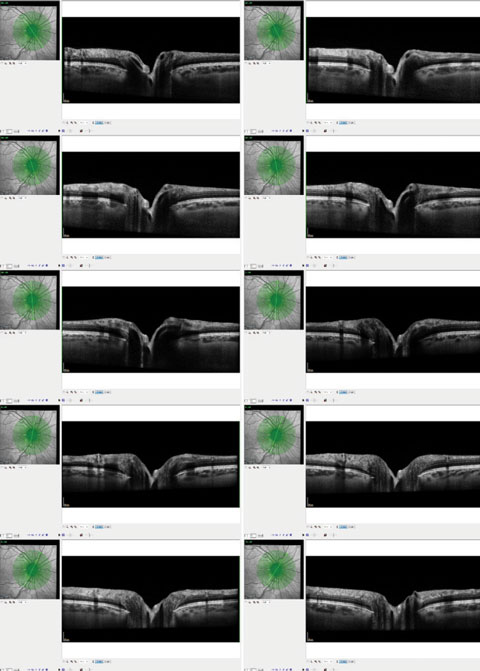 |
| These OCT images show radial scanning of the optic nerve and identify the edge of Bruch’s membrane. High resolution of Bruch’s membrane opening gives us a true picture of the actual optic canal, and subsequent measurements of the rim with in these areas is precise and repeatable. |
Treatment options were limited at that time. Timolol was the workhorse of topical therapy, and Propine (dipivefrin, Allergan) had only recently been approved. Of course, pilocarpine and other cholinergics were available, although accompanied by associated side effects. Often, patients we treated ended up undertreated, and those we only monitored eventually developed field defects detectable with standard automated perimetry.
Eventually, we recognized that glaucomatous optic neuropathy did occur in the early stages without identifiable visual field loss and, subsequently, the Academy of Ophthalmology changed its definition of glaucoma by removing the recommendation that field defects be present.1 Given that field testing was subjective and variable in reliability, we tended to rely more on structural appreciation of optic nerve nuances and IOP in determining the presence or absence of glaucoma. Stereoscopic optic nerve photography was considered the gold standard in optic nerve imaging, and it served us well.
We Have the Technology
The early 90s saw a movement to develop more precise instruments to measure optic nerve characteristics. Visual field testing modifications remained relatively stagnant. Also, when these newer imaging instruments were becoming more common, the results of several well-designed glaucoma risk factor studies began to trickle in. These are now commonly referred to as the “alphabet soup” studies of glaucoma, due to their names—“The Ocular Hypertension Study (OHTS),” “Advanced Glaucoma Intervention Study (AGIS)” and the “Collaborative Initial Glaucoma Treatment Study (CIGTS),” for example. Further studies on the data they presented have left us with good guidelines on how to evaluate a patient with glaucoma and predict their likelihood of progression.
While the imaging technology began to take on a more precise, objective nature, we as clinicians tended to describe the optic nerve in simple terms related to the relationship between the optic disc and the optic cup; the all too familiar cup-to-disc ratio. While the use of the cup-to-disc ratio was a simple tool to describe some characteristics of the optic disc, we relied too heavily on its documentation. We’ve all had patients for whom we document a cup-to-disc ratio widely different from one visit to another. We may see a nerve and call it 2x2 then, the next time we see the same nerve, call it 1x1. Of course, inter observer variation is even greater. So while we’ve realized that the cup-to-disc ratio has limited practical value, we continue to use it. And even objective instrumentation, whether it’s scanning laser tomography or optical coherence tomography (OCT), usually has some reference to a ‘cup’ and ‘disc’ in one form or another.
With the advent of high resolution OCT technology, some researchers have suggested modifying our approach to evaluating the optic nerve by including different markers of optic nerve structure, such as Bruch’s membrane opening.
 |
| These OCT images show radial scanning of the optic nerve and identify the edge of Bruch’s membrane. High resolution of Bruch’s membrane opening gives us a true picture of the actual optic canal, and subsequent measurements of the rim with in these areas is precise and repeatable. Click to enlarge. |
The World of Tomorrow
At the end of the day, anatomy is anatomy is anatomy. Knowing normal anatomy, and the finer nuances thereof, makes identifying abnormal anatomy much easier.
When we look at a cross section of the optic nerve, all individual ganglion cells (whether there are a million of them or only 100,000), pass from the retinal ganglion cell layer into the optic nerve by passing medial to Bruch’s membrane opening.
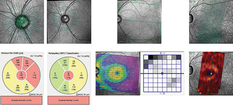
So where does this lead the clinician in a glaucoma practice? One study shows rather exquisitely the relationship between the Bruch’s membrane opening (BMO), the internal limiting membrane and the neuroretinal rim of ganglion cells that lies between these two readily identifiable structures.2 By identifying the BMO, and the adjacent neuroretinal rim in a series of cross sections through the optic nerve, a viable picture begins to emerge of the volumetric characteristics of the very ganglion cells we are trying to salvage.
Furthermore, retinal nerve fiber layer (RNFL) circle scans centered around the optic nerve can identify areas of nerve fiber layer thinning corresponding to preferential areas affected in glaucoma.
Likewise, studies show defects in the ganglion cell layer in the macula, indicating early glaucomatous structural loss.
But the central question remains unanswered: where does the structural loss initially occur? In the macula? In the perioptic RNFL? How far away from the center of the optic disc should we measure the RNFL? Does it occur first in the neuroretinal rim in the optic disc adjacent to Bruch’s membrane opening? We don’t know the precise answer yet—my guess is that it can occur in any of these locations first, probably governed by individual patient characteristics. With that being the case, we need to image all these areas.
Functionally, some newer perimetry strategies and instruments better correlating with early detection are evolving. We will be seeing more developments in the next few years, as more data comes in pertaining to new, more reliable scanning techniques. Eventually, we will begin easing away from the cup-to-disc terminology that we’ve held on to for decades.
|
1. Glaucoma Research Foundation. What is the definition of glaucoma? Available at: www.glaucoma.org/q-a/what-is-the-definition-of-glaucoma.php. Updated: August 27, 2012. Accessed: September 1, 2016. 2. Reis A, Sharpe G, Yang H, et al. Optic disc margin anatomy in patients with glaucoma and normal controls with spectral domain optical coherence tomography. Ophthalmology. 2012 Apr;119(4):738-47. |