 |
A 54-year-old Caucasian female was referred to determine whether she should be treated for glaucoma. The referring provider did a great job in the preliminary evaluation, obtaining multiple IOP measurements over a three-month period, visual field studies, OCT imaging and gonioscopy, yet the question remained to begin therapy or not.
Patients like these are seen every day in glaucoma clinics and, in many cases, the decision to begin intervention or passively monitor is based primarily on clinical judgement.
 |
| Fig. 1. Several metrics are available for evaluation of a glaucoma suspect, including the ganglion cell layer analysis and the RNFL analysis. Also noted are disc topography metrics. Click image to enlarge. |
The Case
This particular individual was taking no meds other than vitamins and OTC supplements and reported no allergies to medications. There was the possibility of a history of glaucoma in her family, but the details were not clearly elucidated. Entering visual acuities through mildly hyperopic astigmatic and presbyopic correction were 20/20 OD, OS and OU. Pupils were ERRLA with no APD, and EOMs were full in all positions of gaze. The patient was not refracted, as the purpose of the initial visit was a second opinion regarding glaucoma.
Previous IOP readings were, on average, 24mm Hg OD and 25mm Hg OS, as reported by the referring provider. We obtained similar IOPs of 23mm Hg OD and 24mm Hg OS. Previous pachymetry readings were 540μm OD and 533μm OS, again consistent with our readings. Threshold visual fields were normal.
A slit lamp exam of the anterior segments was essentially unremarkable, with clear corneas, quiet chambers, open angles and no transillumination defects or Krukenberg spindles OU. Gonioscopy demonstrated wide open angles with a flat iris approach, minimal trabecular pigmentation and no angle abnormalities.
Through dilated pupils, the patient’s crystalline lenses were clear OU. Stereoscopic examination of her optic nerves demonstrated a cup-to-disc ratios of about 0.40 x 0.35 OD and 0.40 x 0.40 OS. The neuroretinal rims were plush and well perfused and deemed to be of average size. Her retinal vascular evaluation was entirely normal, as was her macular evaluation. Mild vitreous syneresis was observed. Her peripheral retinal evaluation was unremarkable.
 |
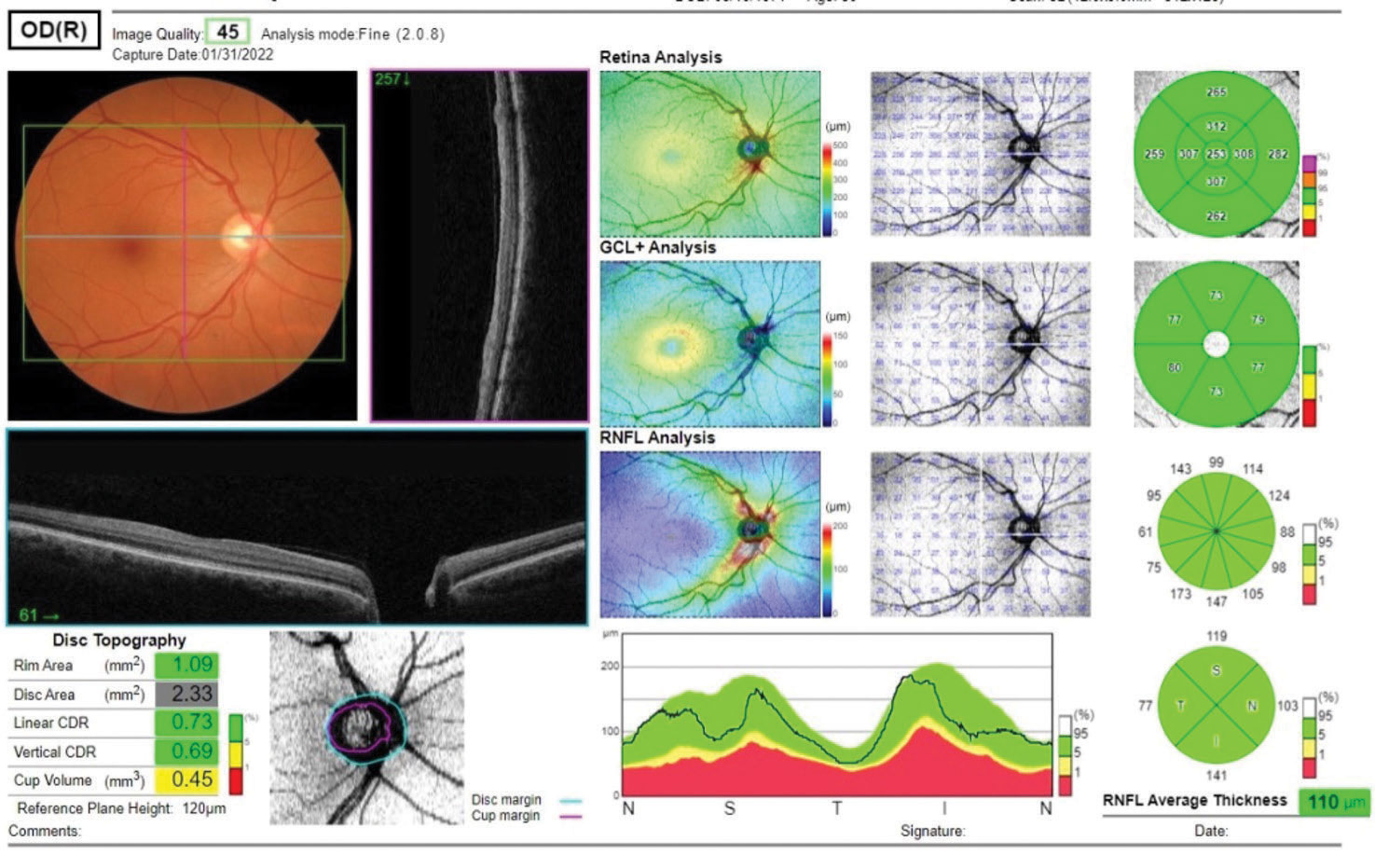
| Fig. 2. The reference database plots of the patient’s RNFL circle scan in an NSTIN format. Metrics of the right optic nerve raised questions; namely, a larger cup-to-disc ratio than seen clinically. Click image to enlarge. |
Discussion
With a questionable family history of glaucoma and IOPs in the mid-20s, certainly there is a risk for glaucoma. But what was most concerning for the referring provider were some of the OCT findings obtained; namely, the optic disc metrics.
It’s common knowledge that different providers subjectively looking at the optic nerves of the same patient may very well judge the cup-to-disc ratio differently. This inherent confounder is common, especially when you see a patient of a previous provider. This was the case with the referring provider, as they had inherited the patient from another OD who had their own method of interpreting her optic nerve characteristics.
Naturally, with the heavy reliance on OCT technology in evaluating glaucoma patients, much of the subjectivity of optic nerve parameters is eliminated by the objective measurements that OCT provides. However, the interpretation of these objective measurements remains subjective in nature, and different clinicians looking at the same OCT readings may come to different conclusions.
This is one of the reasons why you need to know and thoroughly understand the details that your OCT technology is providing you. I’ve previously mentioned the tendency to overly rely on reference databases and cautioned against doing so. But what happens when some of the OCT findings are suggestive of the presence of disease while other parameters are not? This is where your interpretive skills come into play, and those skills must be shaped by an understanding of the information the OCT provides.
At the end of the day, there are many very good OCT devices on the market, and they do provide reliable data that is objective in nature. How they generate that information varies somewhat from company to company; thus, understanding how your particular instrument processes data is critical.
Of course, OCT’s evolution has moved from a single analysis of the circumpapillary RNFL thickness to analyses that include not only the RNFL but also the macular ganglion cell layer, as well as metrics associated with the optic disc itself. When these objective findings match our subjective finding from the physical exam, formulating an assessment is easy. But when they don’t, then we must use our clinical judgement.
The majority of the OCT findings in this patient are representative of a healthy glaucoma suspect (Figure 1). The RNFL metrics are good, as are the ganglion cell metrics. With a cursory view of the OCT report, there may not be any suspicion; however, after closely examining the optic nerve metrics, a different picture emerges (Figure 2).
While both my and the referring doctor’s physical exam of the right optic nerve seemed to indicate a relatively healthy appearing structure, the OCT results demonstrated a different interpretation of the cup-to-disc ratio. And this is where the devil is in the details. As we move away, gradually and albeit slowly, from using the subjective cup-to-disc ratio as a solid metric on physical exam, OCT—by its inherent objectivity—aims to provide a reliable and repeatable metric of the cup-to-disc ratio, unbiased by subjectivity. But we need to keep in mind how OCT calculates this ratio and recognize that each OCT does it differently.
The basis of OCT interpretation of the optic nerve itself, and namely the neuroretinal rim tissue, is predicated upon identification of Bruch’s membrane opening (BMO), which frankly is very easy with OCT. The BMO is not identifiable at the slit lamp. Essentially, the BMO is the de-facto limit of the optic canal. In other words, all axons of ganglion cells exit the eye at the optic nerve medial to the BMO, making this structure the passage through which the axons are traveling. When an OCT calculates cup-to-disc ratio, this is effectively the optic disc size.
But what about the cup size? How is that determined? Again, the devil is in the details. I’ve heard comments from some providers who are not fond of OCT’s generated cup-to-disc ratio. The reasons cited are often related to the ratio not matching the in vivo appearance. In many instances, they won’t match up, especially since we can’t see the BMO in vivo at the slit lamp.
With the Maestro OCT (Topcon) used in this case, the calculated cup-to-disc ratio is based on the BMO and a plane 120μm anterior to the BMO. The cup size is larger than our subjective in vivo estimation (Figure 3).
It is very important to note that the BMO generally does not change over time, whereas—should glaucoma progress—the neuroretinal rim would thin and, thereby, the OCT-calculated cup-to-disc ratio would naturally enlarge. But the disc itself does not enlarge. And therein lies the value of the OCT-calculated ratio: it readily shows change should the disease progress. And given the technology’s resolution, that change would be visible on OCT well before we would see it in vivo.
Where the difficulty comes in is in the initial set of scans, especially if our subjective interpretation of the cup-to-disc ratio differs significantly from the objective ratio calculated by OCT, as it does in this case. Don’t dismiss the calculated cup-to-disc ratio in these cases, as we cannot visualize in vivo the BMO, while OCT can. But do use the OCT-generated ratio to assess for change over time, which is what we are all looking for in the long-term management of our glaucoma patients.
 |
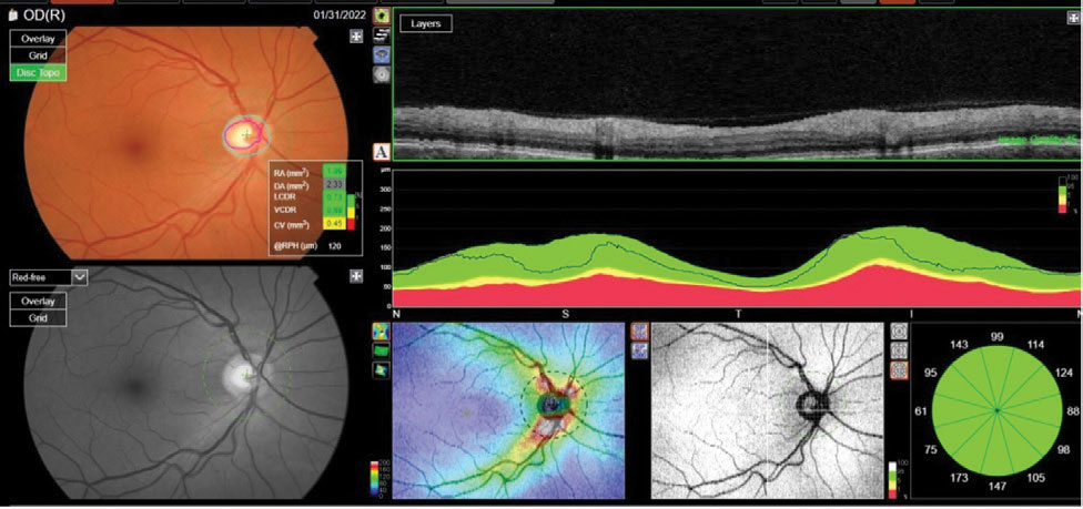
| Fig. 3. The BMO is identified by the horizontal green line (connecting the lateral edges of the structure) and the cup edge is identified by the purple dots. The cup edge is on a plane 120μm anterior to the BMO plane and extends laterally from the edges of the axons exiting the nerve. Click image to enlarge. |
Takeaways
So, what is this patient’s diagnosis? I believe she is a glaucoma suspect with no frank OCT or visual field evidence of damage; therefore, she will only be monitored. While the OCT results seem to conflict with our exam findings, they just present the case in a different fashion than we can see in vivo.
Moving forward, the patient will be seen by the referring provider who will ultimately be looking for progression on OCT in the macular ganglion cell layer, RNFL and neuroretinal rim cup-to-disc ratio.
Dr. Fanelli is in private practice in North Carolina and is the founder and director of the Cape Fear Eye Institute in Wilmington, NC. He is chairman of the EyeSki Optometric Conference and the CE in Italy/Europe Conference. He is an adjunct faculty member of PCO, Western U and UAB School of Optometry. He is on advisory boards for Heidelberg Engineering and Glaukos.